The Normal Distribution—How Chance Can Be Calculated.
The scattering of random factors follows mathematical laws that are described by distribution functions. Because of the properties of these functions, it is possible to calculate the probability of occurrence of individual values. Of all the distribution functions, the normal function is probably the most important because it can be used in a wide variety of applications.
It would be great if you could influence the coincidence.
You would adjust the randomness to make as much money as possible.
Regarding fuel economy, you would set all the random consumption factors for the lowest fuel consumption.
… but that is unfortunately not possible!
You can only change the systematic consumption factors, you have no influence on the random factors. Chance doesn’t listen to you!
But did you know that chance still follows fixed laws?
Even if you have no control over chance, it still can’t do what it wants. The universe has rules, chance must obey, and scientists have figured them out.
Here in this article, I explain these rules.
We’ll look at what we can find out about the occurrence of random factors.
With this knowledge, you can create a single representative value from your many different fuel consumption values.
You can use the standard deviation to evaluate the spread of your fuel consumption values and assess the quality of your average consumption value.
You can find out why and how fuel consumption varies in the article: »Why does fuel consumption vary? (a simple explanation)«.
The application of the theory to fuel consumption determination using the fleet monitoring method can be found in the article: “How to assess the distribution of fuel consumption values.” which I am going to publish soon.
Without further ado, let’s get started right away.
It happens by chance.
Something that happens by chance was not planned by anyone.
Source:collinsdictionary.com
I think in English, there are different words when something happens without intention or without the possibility of someone’s influence.
- Chance
- coincidence
- accident
- fortuity
- happenstance
- randoms
In the physical-technical context, we are often confronted with the outcome of complex systems. Systems, that are so complex or unexplored that we don’t understand their behavior. Therefore, we are not able to predict their outcome, nor do we have the ability to influence the outcome in any way.
It means those things are beyond our control.
That’s why things happen randomly. Random outcomes are distributed over a range or are repeated.
At the same time, these random outcomes are the input for other systems that we are interested in.
Therefore, it is important to understand randomness in order to assess its impact.
What is a distribution?
The distribution of a random variable shows the frequency of occurrence of the individual values in a series of measurements or a data set.
I have brought you a chart for illustration, in which I have shown the distribution of my car’s fuel consumption values. (Yes, I have to admit, it wasn’t exactly a small car.)
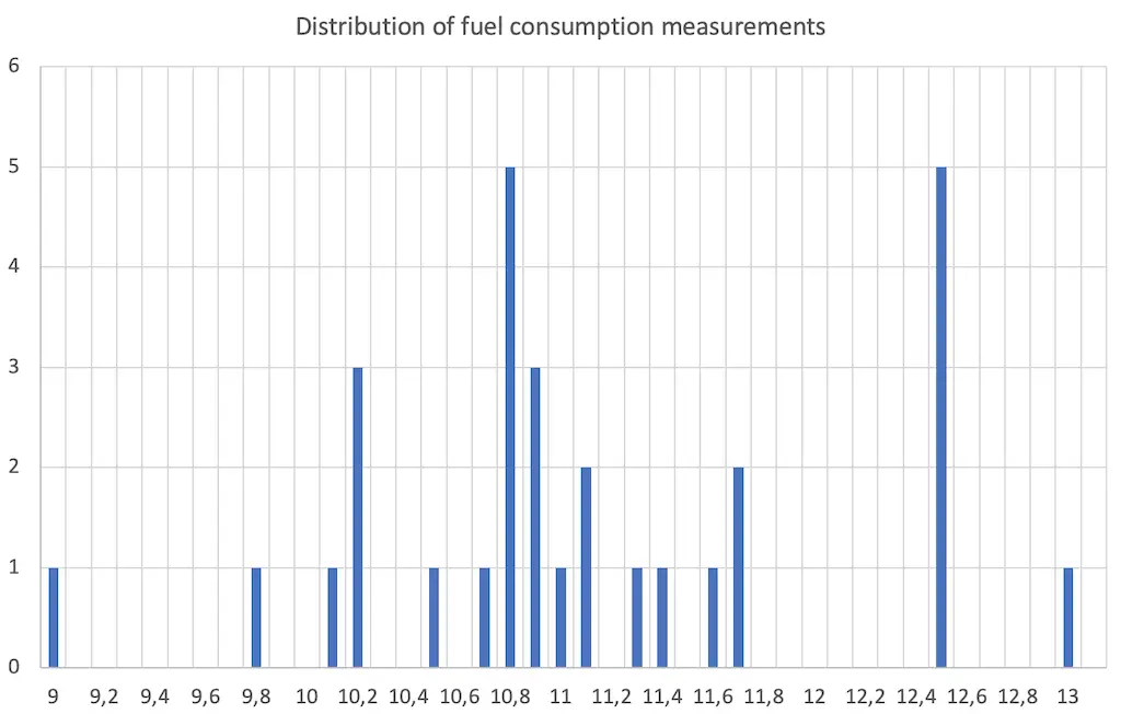
The fuel consumption values can be found on the horizontal axis and the frequency of occurrence on the vertical axis.
You can see that in my series of measurements, some consumption values did not occur at all. 10.8 and 12.5 l/100 km have each been measured 5 times and are therefore the most common values.
Apart from the knowledge that consumption values between 9 and 13 liters per 100 km were calculated, this representation does not make us much smarter.
This is because I only took 30 readings.
If I had made an infinite number of measurements, then we would be able to see a mathematical function in this representation.
This is a typical problem. We have to find another way of finding out our function.
A distribution function tells us the probabilities of occurrence.
Distribution functions describe the mathematical law according to which the frequency of random values occurs.
The probability of occurrence of random variables can be described mathematically using distribution functions.
This is useful for us. If we know the distribution function according to which a random variable is distributed, then we can find out the probability of the occurrence of individual values. Even if we have only a limited number of measured values.
You can see the most important distribution functions on the Analytics Vidhya website: “6 Common Probability Distributions every data science professional should know”
If you look at the functions, you will see that the distribution of the values in the different cases is very different.
Unfortunately, the uniform distribution applies to lottery games. With this distribution function, the probability of occurrence is the same for all values. Knowing this distribution function will not make us a lottery millionaire.
This is different for the normal distribution, there we have values that occur much more frequently than other values. And fortunately, the normal distribution applies to fuel consumption.
What is a normal distribution?
The normal distribution is a distribution function that often occurs when many randomly scattering influencing factors affect a situation. The type of distribution of the individual factors is irrelevant.
Quelle: Uni UlM
You can see the mathematical proof of this definition at the link to the source. The mathematicians use the central limit theorem to prove this. But you can also just believe it because for a non-mathematician this is a very demanding material.
Since there are regularly such situations with many random influencing factors, the normal distribution is very often applicable. Here are some examples of normally distributed problems:
Many random influencing factors also have an impact on fuel consumption.
We can assume that the distribution of fuel consumption values follows a normal distribution.
This is great because the normal distribution has properties that will help us a lot.
Who discovered the normal distribution?
The German mathematician Carl Friedrich Gauss from Göttingen researched the normal distribution and its characteristic parameters.

His discovery was groundbreaking for mathematics and still helps us today to answer very, very many practically relevant questions.
Because it is so common, this distribution has been given the name “normal distribution”. (According to the motto: Normally you can use this function.)
The merit of Gauss is so great that the normal distribution is called “Gaussian distribution”.
The importance of his achievement was recognized by the fact that Gauss and his “bell curve” were depicted on the old German 10-mark note. The 10-mark note is a thing of the past, but the importance of Gauss’ achievement has remained.
What does the normal distribution look like?
The normal distribution can be described by two mathematical functions and their function curves:
The distribution function
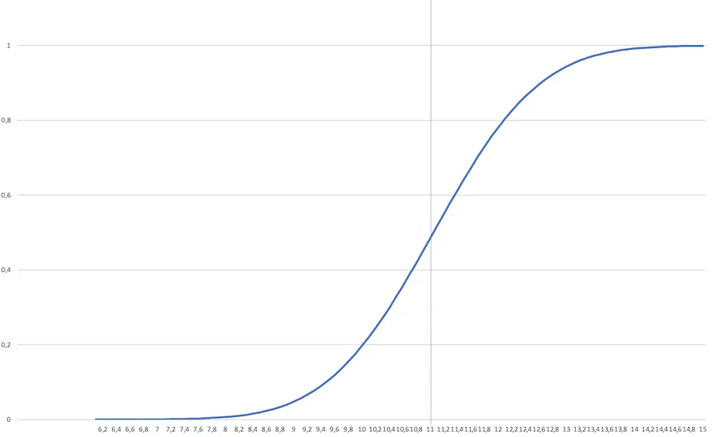
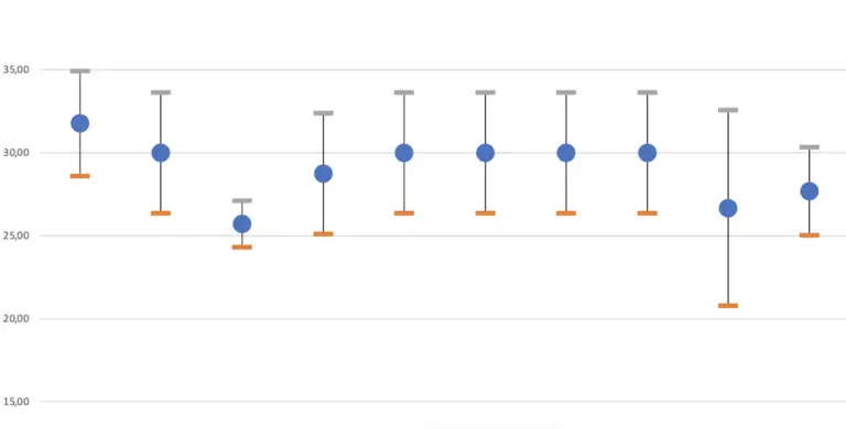
In the picture of the distribution function, you can see the function curve that results when I calculate the normal distribution that matches my measured values.
Let’s have a look at what we can see here.
You see that we can derive additional information from the distribution function. However, this information is not really relevant to practice. That’s why you rarely look at the distribution function, but at the density function.
You may be wondering how I can read that so accurately. Well, I can see that from the table I used to draw the function curve.
The density function
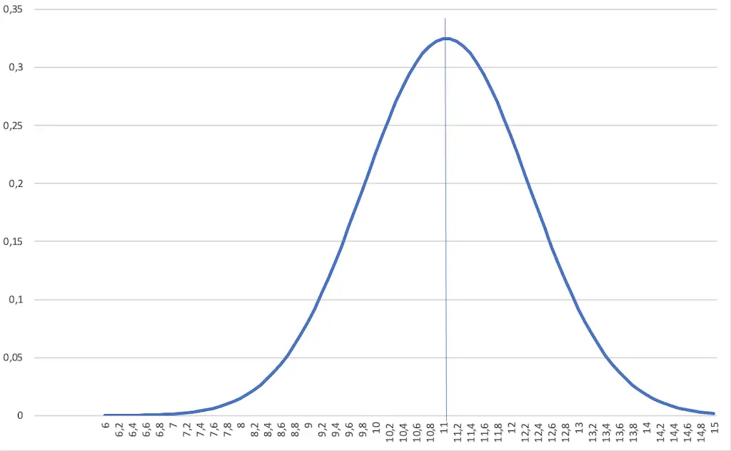
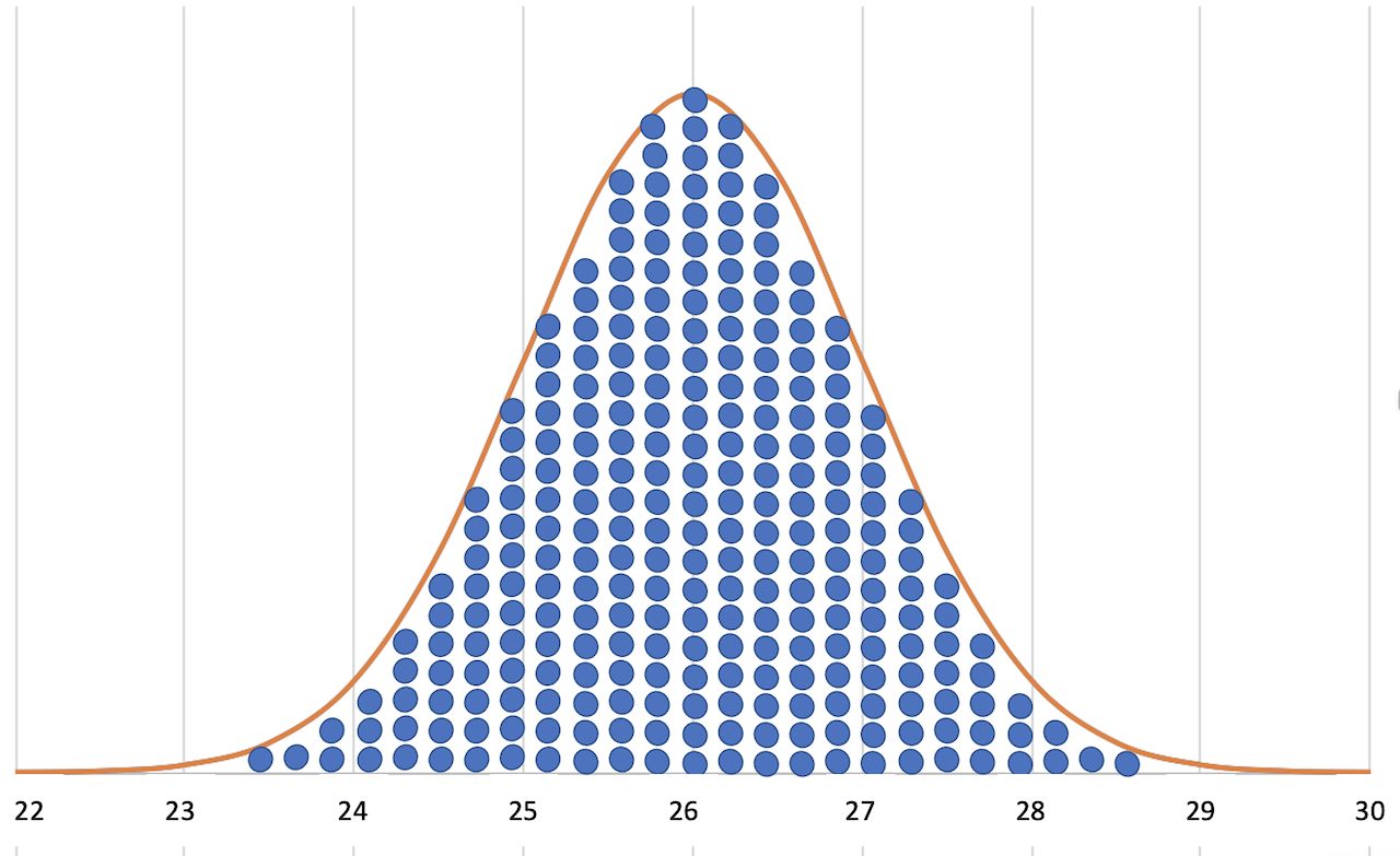
The function curve of the density function is the famous “bell curve”.
Due to its characteristic shape, the density function curve of the Gaussian distribution looks like a bell. It is therefore called the “bell curve”.
As the name suggests, the density function shows how close the individual values are to each other.
If the curve has a narrow, slender shape, then the individual values are close together. This means that the scatter is small and the probability of occurrence of the individual values near the mean value is high.
On the other hand, if the curve has a broad, bulbous shape, then the scatter is large. The probability of occurrence of values that are further apart is similarly high.
The density function of the normal distribution has distinctive features that we will use.
What do the parameters of the normal distribution tell us?
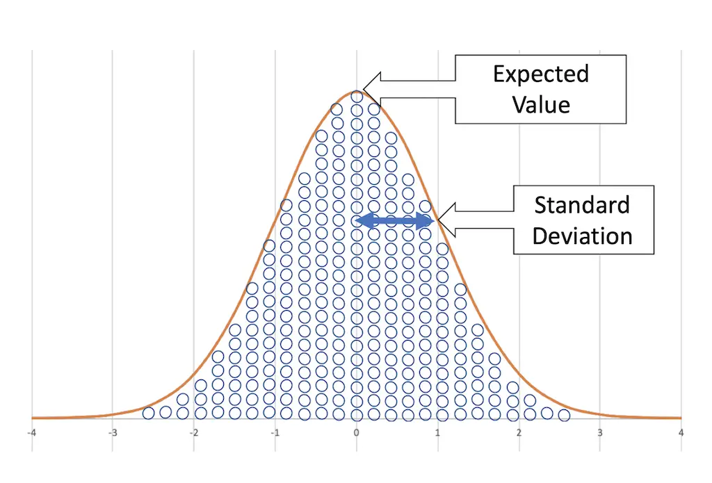
The expected value
The expected value of the density function is both the arithmetic mean and the median of the population of all values of a normal distribution.
The expected value is the value that occurs with the greatest frequency. It represents the average of all values.
Because the curve is symmetrical to the expected value, there are just as many smaller values as larger values. That’s why the values average out and what’s left is the expected value itself.
That’s a huge advantage! This allows us to merge all values into a single value!
This value is what you are looking for when you want to know your fuel consumption.
The many variations that cause variability balance out, leaving a single value to work with.
We can use the expected value because it stands for the pure, non-variable consumption.
The representative fuel consumption value that we want all the time is the expected value of the density function of fuel consumption values.
The true value.
Unfortunately, there is a small but significant catch.
The true mean value will always remain unknown to us.
When we calculate the density function of our normal distribution, we never have all the individual values that belong to our function.
We only ever have a random selection of values. This selection is called “random sample”.
So we cannot be completely sure whether the mean that we calculate is really the absolutely correct mean of the normal distribution.
This value is therefore also called the expected value. We “expect” this value to be the true mean, but we cannot be absolutely sure.
So we have to check how big the possible deviation between our expected value and the true mean can be.
There are formulas that you can use to calculate how large the area around the expected value is, in which the true value is with a certain probability.
But I don’t think that’s very helpful.
A good indicator is the standard deviation because it gives you information about the scatter of the entire distribution and thus also about the uncertainty of your expected value.
The standard deviation
The standard deviation characterizes the bulging of the curve. It represents the turning points of the curve. 68% of the values are within one standard deviation (up and down).
The standard deviation gives us a sense of how the individual values scatter. This allows us to estimate how often values in the range of the expected value occur.
For this reason, we can use the standard deviation as a parameter that shows us the scatter.
The symbol for the standard deviation is sigma. You may have heard of “Six Sigma” before.
Within 6 times of the standard deviation are 99.99966% of the values of the normal distribution. So there are practically no values outside this range.
In quality assurance, one tries to keep the range of deviations from the norm as small as possible. Therefore, a target range for 6 standard deviations of the normal distribution of the value in question is specified. Once that has been achieved, there are practically no more rejects.
For our purposes, one Sigma is sufficient. We don’t want to overdo it.
Drawing the normal function.
In order to get the density function of the concrete normal distribution of your fuel consumption values, you have to calculate the two parameters of the normal distribution.
Since we don’t know the real parameters of our function and will probably never find out, we use a simple trick.
We just take the values we have. We use this to calculate the mean and use it as the expected value. Using the spread formula, we calculate the standard deviation of our sample.
You can find the necessary formulas in the article on calculating the average consumption.
If you now have these two values, you can, for example, have the curve drawn on the Department of Statistics and Actuarial Science
University of Iowa page.
There is a formula in Microsoft Excel that calculates the values of the normal function. It could then look like this:
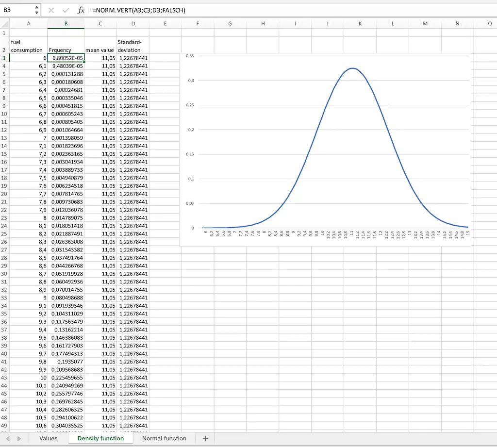
The formula is called NORM.DIST(value, mean value, standard deviation, false). If false you get the density function, if true you get the distribution function.
If you would like to get the pictured file from me, then write me an email and I will send it to you free of charge. I would just ask for permission to store your e-mail-adress so I can inform you about new articles.