How to assess the distribution of fuel consumption values?
The distribution of average fuel consumption values can be assessed by calculating the standard deviation and the confidence interval of the normal distribution.
How accurate is the average consumption you calculated?
Can you trust this value, or is it too imprecise?
These questions mainly arise when you want to compare fuel consumption values with each other in order to draw conclusions from the difference.
If the scatter is too large, it can lead to wrong conclusions. That’s why you need to control the scatter.
In this article, I will explain how you can calculate and assess the standard deviation. You’ll learn why it’s a good measure of variability and how it helps you assess a potential error.
I will also address the confidence interval of your sample. This makes it possible to further narrow down the estimate of a possible error.
To be able to perform the steps presented here, you must have previously collected and calculated fuel consumption values using the fleet monitoring method and calculated your average consumption values from them.
If you haven’t done so yet, feel free to check out the corresponding articles again. The links will take you directly to the respective topic.
At the end of this article, you can order a free Excel tool, with which you can calculate your own values.
An explanation of why fuel consumption scatters in the first place can be found in the article: “Why does fuel consumption vary? (a simple explanation)”.
But now let’s get started.
Why is average consumption not necessarily accurate?
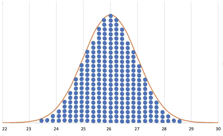
We know that the scatter of fuel consumption values can be represented by a normal distribution function. That’s why you can combine many consumption values into one or a few average consumption values. (Why this is the case, I have described in the article about the normal distribution).
This makes it possible to compare a few representative fuel consumption values with each other.
Now, unfortunately, you never have all the values available for calculating average consumption, which are part of your normal functions.
You only ever have a sample at your disposal.
This can cause a problem with the accuracy of the mean value of the normal function. That’s why we need to take a closer look at this now.
What is a sample?
A sample is:
Duden
1. part of a whole, which came into being after a certain selection procedure,
2. investigation, control of a sample in order to conclude about the whole.
The individual consumption values you collect during fleet monitoring represent a subset of all possible consumption data. Therefore, they are a sample from the population of the distribution function.
And yes, we want to conclude from this example to the whole!
To be precise, it is a random sample. Because the selection procedure is a random selection.
This is good news because random samples are usually less affected by systematic errors. Chance just likes chance.
What is the reason for the inaccuracy of the average consumption?
In a normal distribution, the probability of occurrence of each value is determined, but the order of occurrence is not.
For this reason, it is not known in which order randomness feeds the values into the sample.
If you are lucky, the most frequent values in the normal distribution are also the most frequent in your sample.
The deviation between your mean and the true value of the normal distribution is then small, and you can work with the value without worrying.
But it may also be that chance puts the exotic values on your table first.
Then there can be a significant deviation between the average consumption and the true value of the normal distribution. The value you have calculated (average consumption) then does not represent the totality of all values of the population!
There is no practical way to find out the true value exactly, and thus we cannot say how big the deviation is.
Because the distribution is a normal distribution, you can estimate how large the area around the calculated mean is in which the true value is located with a certain probability.
Which parameters influence the accuracy?
The spread of the distribution.
The extent of dispersion of the population influences the possible deviation of the sample mean.
This scatter comes from the use.
If the conditions during the journeys are always very similar, for example in long haul with a lot of freeways, then the scatter of the values is small.
If the conditions are very different, as for example in use on a construction site, then the scatter of values is large.
It is logical. If there is already a large scatter from the use of the vehicles, then of course the scatter of our sample will also be large.
Normally, we will put up with it.
In some cases, however, it may make sense to create several from one distribution. In other words, you can split the driving profiles and sort these segments according to use conditions.
The number of individual values.
The more values you have in the sample, the greater the probability that the values with a high probability of occurrence will also occur frequently in the sample.
That is also logical again. Chance abides by its own rules.
The standard deviation from the average consumption – a measure of the scatter.
In the article about the normal distribution, I mentioned the standard deviation. It is a measure of the belliness of the density function.
Here we now look at how to calculate it and how it helps us assess the trustworthiness of average consumption.
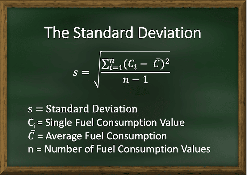
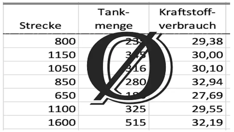
The standard deviation is calculated by taking the difference between each individual value and the mean value. Then square this, add it up, divide by the number of readings minus one, and take the square root.
Fortunately, the standard deviation is available directly as a formula in Microsoft Excel:
=STDEV.S()
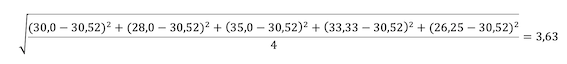
In the article about the calculation of the average consumption, I showed an example in which I calculated the average consumption from 5 strongly scattering individual values. The average value was 30.52 l/100 km.
The associated calculation of the standard deviation then looks like this:
Now you know the mean value (average consumption) and the standard deviation. This opens up two options for you:
- You can plot the density functions of the normal distribution on top of each other and draw conclusions about the possible errors.
- You can calculate the “confidence interval”. This is the area around the mean value in which the true value lies with a certain probability.
You should do the second step if you do not get a reliable result with the first step.
Assess the normal distribution functions.
If you plot the density function curves of the groups of fuel consumption values you want to compare on top of each other, then you can estimate the consumption trend.
Let us now take a look at some possible constellations in examples.
Case 1: The scatter is equal, the average consumptions are further apart than the scatter.
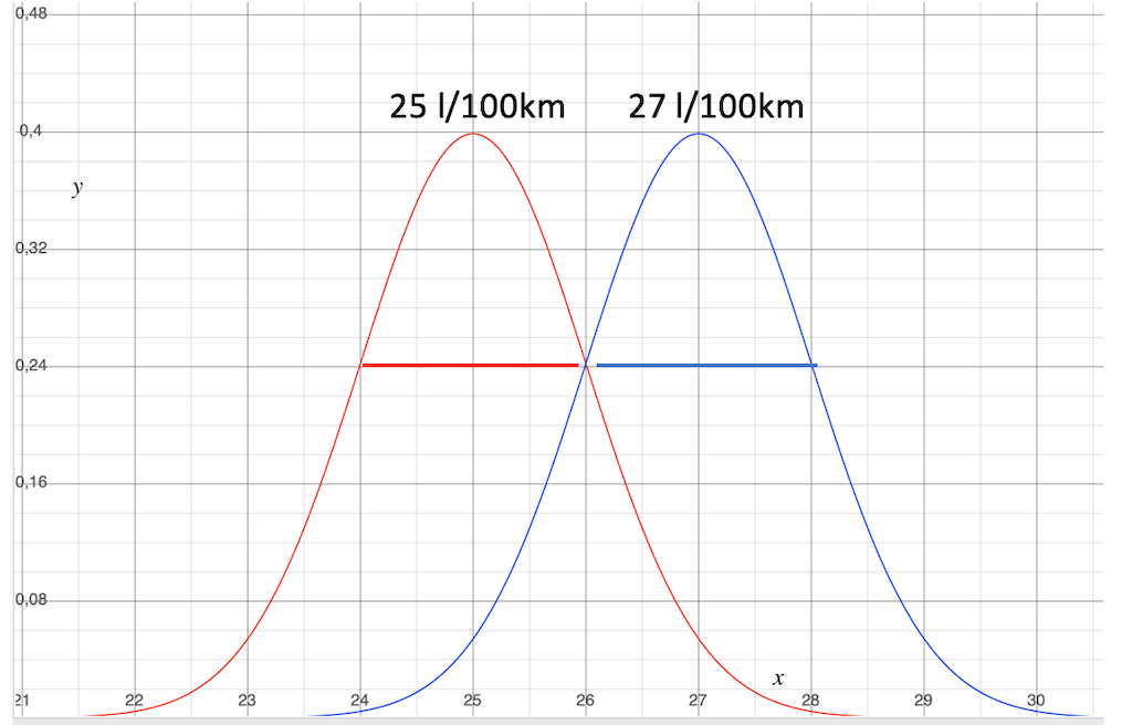
That’s the way we would prefer it to be.
The standard deviation of the two normal distributions is the same, so the spread of the values is also the same. This suggests comparable operating conditions.
The difference between the mean values is equal to or greater than the spread of the two mean values. This means that you can be relatively sure that the consumption of the blue groups is really better than the consumption of the red group.
To find out, you don’t necessarily need this graphical representation. You can also see this by looking at the numerical values of the two distributions.
Now that I’ve shown you the curves, I’m sure you can imagine what that looks like from the numerical values and don’t necessarily have to draw the curves.
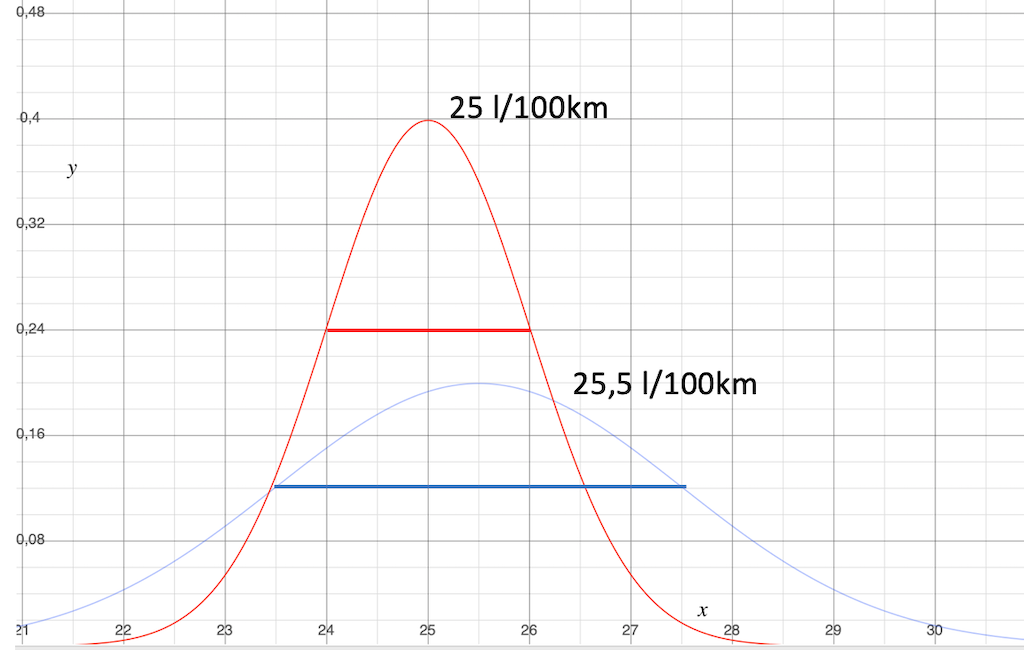
Case 2: The spread is equal, the average consumptions are within the spread.
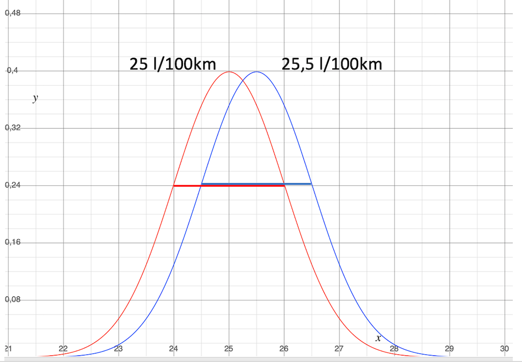
This looks like a need for more analysis.
The standard deviation of the normal distribution is also the same here.
The spread of the values is the same. The operating conditions do not seem to be a problem.
However, the difference between the average values is only 0.5 l/100 km, which is significantly smaller than the spread. Thus, you cannot be sure that the consumption of the blue groups is really better than the consumption of the red group.
- If the true expected value of the red curves lies slightly to the right of the red mean,
- If then the true expected value of the blue curve lies somewhat to the left of the blue mean,
- Then the conclusion is shaky. The consumption difference could disappear or even turn around.
In such a situation, you should be careful with conclusions.
Next, you should calculate the confidence interval.
I’ll explain how this is done just below.
It helps you to further specify the range in which the true value is located. You can then replace the standard deviation with the confidence interval.
If that doesn’t lead to clarity either, you basically have two options:
Case 3: The spread varies, the average consumptions are within the spread.
This situation is something like a statistical SuperGau. We have to pull out all the stops if we want to get a somehow reliable statement at all.
The standard deviation of the normal distribution is significantly different. This forces us to analyze the data in detail.
- Are the operating conditions really so different that such different scattering occurs?
- Does it then make sense at all to compare the consumption values with each other if the use is so different?
- There may also be errors or systematic influencing factors behind this.
Did you forget to write down fill ups? Are there systematic influencing factors that you need to factor out before working with the data?
In such a case, you will have to dive deeper into the analysis of your consumption values and the boundary conditions under which they were generated.
If you find out during the analysis that there are consumption values in the application cases that arose under special circumstances, then sort out these values. This way you can make the scatter more comparable.
At 0.5 l/100 km, the difference between the mean values is again significantly smaller than the spread.
With this, you can’t be sure that the consumption of the blue groups is really better than the consumption of the red group.
Due to the large dispersion, the situation is even more uncertain. So you have to deal with statistics in addition to the systematic factors.
At this point, caution is required in any case. If in doubt, do not draw any conclusions with consequences here.
Calculate the deviation of the average value from the true value.
So far, then, we have estimated how certain the real consumption difference is likely to be.
In practice, I think this will often be sufficient.
However, the mathematicians still have a formula in the program.
With it, you can calculate how large the range around the mean value is in which the true value is located with a certain probability.
Calculate the confidence interval of the normal functions.
The confidence interval around the average consumption
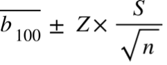
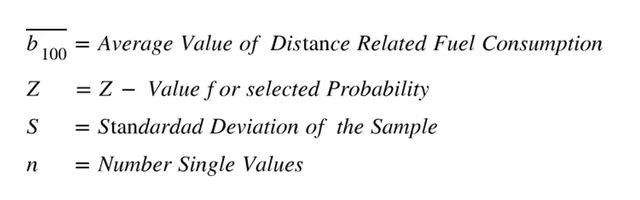
You take the standard deviation of your values and divide it by the square root of the number of values that make up the sample.
Then you multiply by 1.96 and get a range around the mean in which the true value is located, with a probability of 95%.
The Z-value for a probability of 95% is 1.96.
You can use the calculator on this website to calculate the confidence interval.
Here is a brief explanation of the background of this formula:
One can imagine that there are infinitely many samples that can be drawn from one and the same population of the distribution.
The mean values of all these samples are also normally distributed again.
This means that you can calculate a scatter of these mean values.
While the spread of individual values is called “standard deviation” mathematicians say “standard error” for the spread of sample means.
If a probability is added to this standard error, the result is the error margin and a confidence interval.
The confidence interval tells in which range around the mean value the true expected value is located with a selected probability.
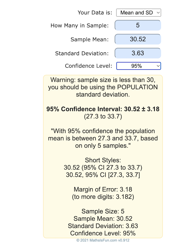
In the article about the calculation of the average fuel consumption, I have calculated the average consumption from 5 strongly scattering single values as an example.
The confidence interval with a probability of 95 % is plus/minus 3.19 l/100 km.

As you can see, this sample is not meaningful even with this approach. No conclusions can be drawn on the basis of 5 values with such a large scatter.
The true average consumption will be somewhere between 27.33 and 33.71 l/100 km, possibly plus/minus 10% away from the average fuel consumption.
This insight is also worth something. I can tell you, I know people who draw conclusions even from a single value and don’t even know what kind of thin ice they are on.
Actually, if I have less than 30 values, I must not calculate with the Z value.
I need a t-value that depends on the number of individual values. Here is a table where you can read the t-values.
To select the t-value, the number of values minus 1 must be calculated. So in our example, I go to the line with the value “4”.
I want the probability 95%, so I go to the column “One Tail 0.025, Two Tails 0.05” (100%- 5% = 95%)
The t-value is 2.776.
So the confidence interval is actually +/- 4.51 l/100 km.
The deviation from the expected value can therefore be even bigger than the standard deviation of the individual values!
In the article about the normal distribution, I used an example from my passenger car, where from 30 individual values an average consumption of 11.05 l/100 km with a standard deviation of 1.227 l/100 km came out.
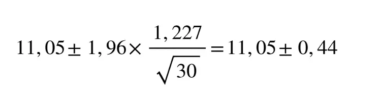
The true average consumption here is between 10.61 and 11.49 l/100 km, which may be plus/minus 4% away from the average fuel consumption.
That is much closer. However, even more, would be possible.
How to improve accuracy?
The miracle cure for improving accuracy is to gather more individual values.
This is again logical, because the more values the sample contains, the more accurate the correct distribution of the values will be.
The values with a high probability of occurrence will grow more than the values with a low probability of occurrence.
Let’s see what would happen if we had more values with the same variation.
| Number of values | confidence interval |
| 5 | +/- 3,19 (4,51) |
| 30 | +/- 1.30 |
| 100 | +/- 0,71 |
| 300 | +/- 0,41 |
| 1000 | +/- 0,23 |
More values in the sample narrow the confidence interval.
This is good because a narrower range means that the probability increases that the mean value is close to the true average consumption.
For demonstration purposes, I have only increased the number of values. Of course, this is not the way it works. You really have to do more driving.
This will additionally reduce the standard deviation of the sample, and make the confidence interval even narrower.
It can also be seen from the table that the accuracy increases less and less as the number of values increases.
This is good news!
It means that the infinite number of individual values in the population can be captured quite well with a few hundred values in the sample.
The systematic error must not be forgotten!
Systematic errors cannot be found with this calculation! Therefore, a further content analysis of the measured values and of the circumstances during the measurement is necessary!
Unfortunately, knowledge of the confidence interval of the average does not mean that major systematic errors may not have occurred.
That’s why you still need to look closely at the values and the operating conditions from which the values come, even if the confidence interval is small.
I have already described some of these possible errors in the articles on calculating the average fuel consumption and measuring distance and diesel volume.
The range of the data is not meaningful information.
Scatter is not to be confused with span.
The span is the range from the lowest to the highest individual value. It is easy to calculate, but says little, since even individual “outliers” strongly influence the value.
That’s good news. We can simply neglect the value that suggests the greatest uncertainty.
My calculation tool for you.
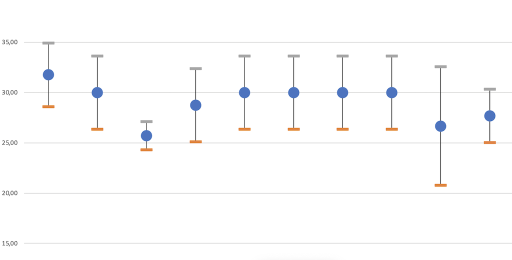
If you write me an e-mail, I will send you an Excel tool for calculating and drawing the distributions and the confidence intervals. You enter your individual values in the group tabs and the table calculates the mean value, total consumption, spread, and confidence interval.
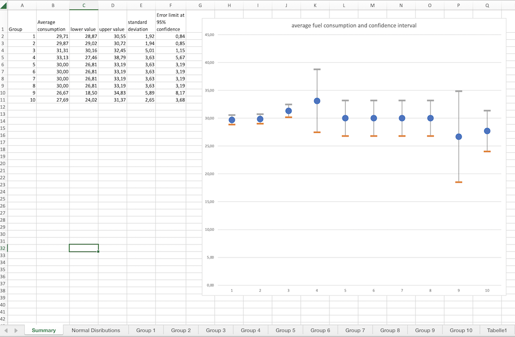
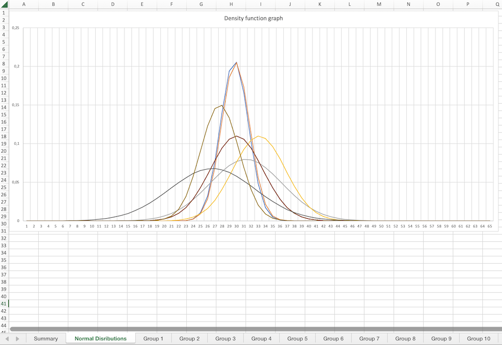
This is how the table looks, you can superimpose several distributions and compare them.
Summary
Please write in the comments how you liked the article and what topics I should still write about.
I guess this article is one of the more complicated ones. If you had difficulty understanding some parts of it, please let me know. Then I can try to formulate this somehow more simply.